Introducing The GMR6000
By Dr. Matsakis
The story of technology is the story of improvement. Every genuine innovation requires a combination of better design and a deeper understanding.[1]. Masterclock's new disciplined oscillator, the GMR6000, is no exception. As successor to the GMR5000, the GMR6000 features a new level of resiliency with power redundancy and a fast-disciplining rubidium oscillator capable of high-precision holdover. We've designed the GMR6000 to utilize its internal oscillator as the source of all output time and frequency signals. As shown in Figure 1, the oscillator gets its time and frequency by adjustments (steering) to bring it in agreement with a reference that could be any of a variety of time sources, including but not limited to GNSS[2].
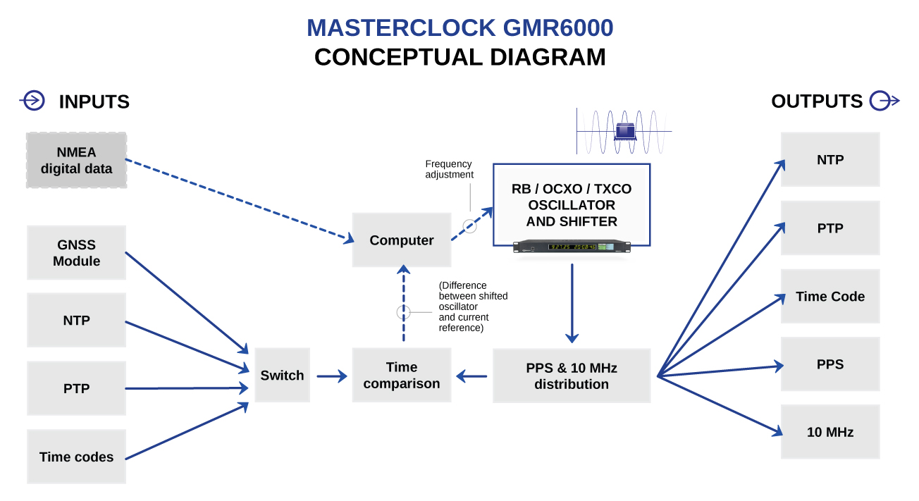
Figure 1 Conceptual diagram of the GMR6000. Time and/or frequency from any of the inputs on the left is compared to that of the oscillator. The oscillator is adjusted to follow the inputs, and the oscillator's output is sent to the users by any or all the means on the right.
The details behind the figure itself could be the subject of many blogs, but this blog is only about the first part of the first step in deciding how to steer the frequency of the oscillator (shown in the top center of the figure). That very first part is to figure out exactly how far off the oscillator's time is from the reference, such as GPS. The better we can model the oscillator, the better we can predict how the oscillator will evolve when the reference is not available (holdover). To model the oscillator, we use past data of the oscillator's time against the reference's time. To test our model, we see how well it can predict the oscillator’s future time against the reference.
For the oscillators in question and for holdovers of a few days, the assumption of parabolic behavior is fairly valid. In that case, a parabola that describes the state of the oscillator can be specified by three parameters: time offset, frequency, and frequency drift. The goal of the math is to find the parabola that best fits the data— given the jitter and quantization noise in the time measurement and the oscillator’s instabilities. Centuries ago Gauss figured out how to do it when the noise is purely random jitter and the oscillator perfectly stable[3]. His idea was to find the curve for which the sum of the squares of differences between it and the data points is a minimum, as depicted in the left side of Figure 2:
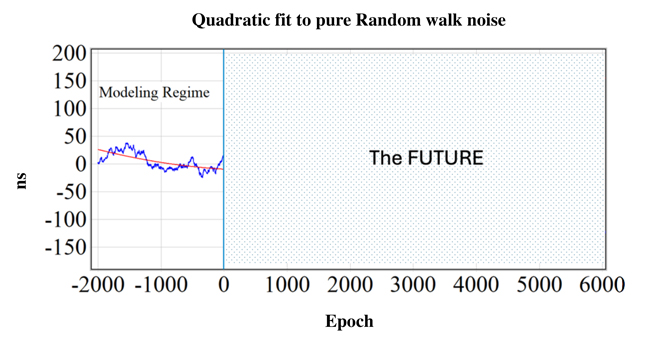
Figure 2 The curved line is the parabola that best fits 2000 data points, in the sense that the sum of the squared deviation of each datum from the curve is a minimum (i.e. as small as it can be.)
It is obvious in the figure that the noise in the data isn't truly random. The points don't just scatter; they walk around a bit. In fact, this is called random walk noise. Random walk is what you get when each data point is the sum of all the truly random jitter from the start to the present[4].
But how good is the least squares fit for predicting? Well, in this example the best-fitting parabola did pretty well at first, and not-so-well later (Figure 3).
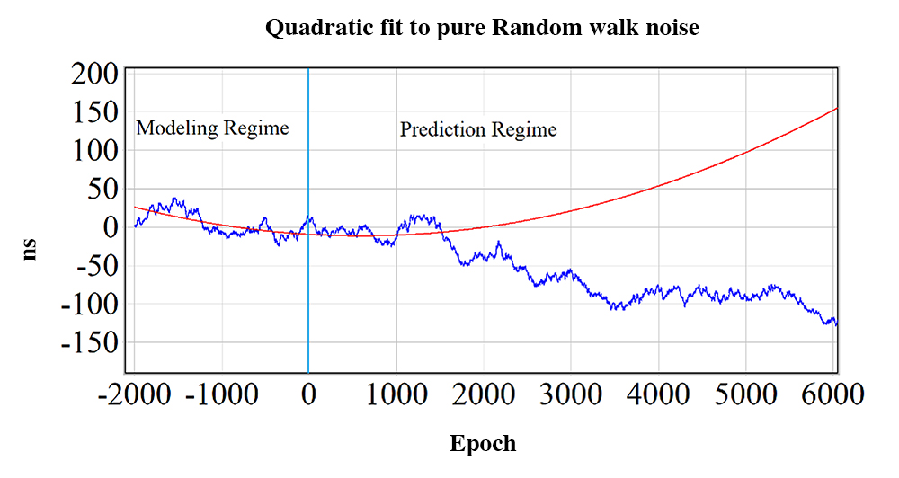
Figure 3 The parabola that best fits the first 2000 points is extrapolated to the future.
This begs the question: how many data points should we have used to fit the parabola for best results? We could have averaged down the noise if we had used more than the 2,000 in the example. But we might also have been more vulnerable to the long-term variations of the random walk, as is apparent in the last half of the data in the figure.
In our 2025 PTTI paper[5], Masterclock Engineer Matt Slavney and I illustrated that the amount of data you need depends on how far in the future you want to optimize your prediction. It also depends on the stability of the oscillator. In the case of an oscillator whose frequency is dominated by random walk[6], we found that you need about as many points in your fitting baseline as you wish to predict into the future. Without enough points in your baseline your accuracy goes down. Ditto for too many. This plot of inaccuracy versus ratio of prediction distance to fitting points says it all:
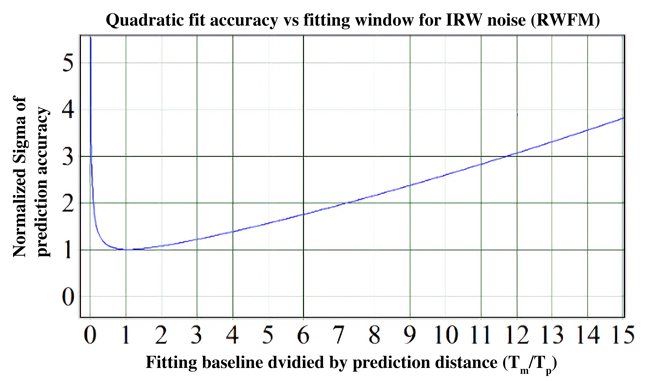
Figure 4 The parabola that best fits the first 2000 points is extrapolated to the future.
But another question is whether we really want to do least squares, as Gauss envisioned it? What about Kalman Filters[7]? In essence, Kalman filters are just least squares being done one datum at a time. This gives the option for the state parameters to evolve between measurements. And the filter doesn't have to retain the old data points because it only uses the current values of the parameters and their current uncertainties. This reduces the computer requirements for memory and speed.
To explain Kalman filters, I like to say they handle parameter-solving the same way people think they think about something in their in daily life. For example, if today you asked Professor Kalman's Swiss granddaughter what Saint Louis was like, she might hazard a guess that it was probably a pretty good place because it was once called the "Gateway to the West", and because it has Washington University, with its GPS-timed NTP server. But she likely wouldn't have a strong opinion until you convince her to visit. Then her opinion would grow as she marveled at the Gateway Arch and strolled through the Botanical Gardens. And imagine when she got to the suburbs and visited Masterclock’s headquarters :) Armed with this new data, she would upgrade her opinion of St. Louis as to being a very, very, very cool place. And she would believe it quite firmly. That's how a Kalman filter works, except that it uses equations instead of neurons. With each new datum it revises its opinion of the parameters that define the clock's state. The new datum would get high weight if the state parameters were poorly known and/or if the uncertainty of the new datum was very small. Otherwise the filter will give the datum less influence on the parameters. Either way, the filter will reduce its inaccuracy estimate. But it will then increase its inaccuracy measurement over the time it takes to get to the next measurement. That makes sense because one must allow for the possibility that St. Louis might have gotten even better since the last visit. (It could also have gotten worse, but let's not think that way.)
Knowing all this, Matt and I compared the predictive inaccuracy of least squares to that of a Kalman filter. In Figure 4, the blue line is the inaccuracy of a Kalman filter and as you can see it is always lower (better) than the others. The inaccuracy of the best possible least squares (with baseline equal to the number of epochs into the future) is in red. But if you want to predict one day into the future you need to store 86,400 one-second points. Storing that much information would raise the cost. Worse, grinding through all those numbers would take too long as well. Decimating the data is an option, and the green curve shows how much higher inaccuracy would be if you were to only store the most recent 100 points.
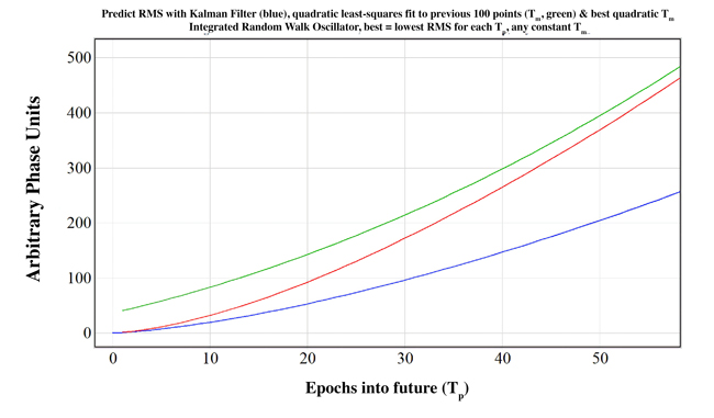
Figure 5 Predictive inaccuracy of a Kalman filter (blue) versus that of optimal least squares (red) and that of a least squares fit to 100 points (green). In this figure down is good.
Figure 5 makes it seem obvious that the Kalman filter is the way to go[8]. So why don't all other companies use them? Maybe it's because Kalman math is out of the designers' comfort zones. But in full disclosure there is another problem. No equation or formula is better than its assumptions, even a Kalman filter. For it to work as well as shown in Figure 5 you need good values for the magnitude of the measurement noise and for the noise characteristics of the oscillator. You need those so you can know how much to allow each new datum to change your estimate of the clock state parameters. For example, if the measurement noise were seriously underestimated the filter would believe each new datum more than it should, and the derived parameters would jump around following the measurement noise. Much the way a "mistuned" person might jump to a new opinion of St. Louis every time it rained. On the other hand, overestimating the amount of measurement noise means the filter would not change its parameter estimates enough. We all know people who won't change their mind when presented with conclusive facts. In our PTTI paper, Matt and I give examples of how Kalman filters could go wrong if you misestimate those things, even though we claim to know how to do it right.
One last consideration is that all the formulas and reasoning given so far apply to an unsteered oscillator. But the oscillator is constantly being steered when in operation with a reference. Those frequency adjustments that we put in obscure the oscillator's variations. The solution for ordinary least squares is to first remove the effects of all previous steers, then find the curve that best fits the unsteered points, and finally to generate predictions by adding the steers back. For a Kalman filter, it is simpler. Each steer can be taken into account when modeling the state parameters' evolution from each measurement to the next. A Kalman filter also allows for future improvements because more parameters can always be added to model any physical effect that might perturb the oscillator.
There is much more to say about the GMR6000's time delivery. For example, after estimating how far the oscillator is off from its reference, you need to decide how rapidly to steer so as to bring it in line. Steering that is too strong would lead to zig-zagging, just like turning the steering wheel on a car would. Gentler steering would more smoothly adjust the oscillator's time and frequency, but the gentler your steer the longer it takes to approximate the reference. Fortunately a theory exists so we can set our steering strategy in the manner best for our application, which is termed the "critical gain"[9].
This is just the beginning for our GMR6000. There are indeed even more advancements being researched and development by our team of engineers. Be on the lookout for additional blogs as we continue to enhance our flagship product with future firmware updates.
Footnotes
[1] Even concrete has a high-tech side. "Ultra-high performance" concrete can use polymer fibers for strength, self-heal with encapsulated healing agents such as bacteria, and reduce global warming using a carbon-catcher for even more strength. However, even today we are just beginning to figure out how to make composites as resistant to sea water as in Roman times.
[2] Technically GNSS stands for any or all of the four Global Navigation Satellite Systems currently in use, one being GPS. But we take this term to mean those and/or any of the many regional enhancements.
[3] One cannot say too many good things about the brilliant Gauss, who lived from 1807-1855. Don't ask me, ask the Wikipedia. His work on statistics has been greatly advanced, and complemented by an understanding that outliers can be more than simple errors to be discarded. Even though statistically unlikely, they can point to a new reality. Like the occasional big shift in the stock market, the appearance of new life forms such as Artificial Intelligence, or even black swans, as the eponymous book by Nassim Taleb expounds upon so well.
[4] George Gamow, probably the only hero of mine who did not die prematurely, called it a drunk-man's walk. That's because a truly drunk person presumably takes each step in a random direction. The steps will eventually lead away from the starting point in some direction or other, in the jittery manner of Figure 2. Random run I guess could be called a drunk-man's driving. Life for engineers would be much better if that kind of noise could be banned.
[5] See Matsakis and Slavney, "Optimal oscillator modelling for GNSS-disciplined clocks on holdover", Proceedings ION-PTTI-2025.
[6] In terms of time, a random walk in frequency is an integrated random walk. It is also termed random run. And what I call jitter is termed white noise, in analog to the colors of light. If you express white noise mathematically as a sum of sine waves, the high-frequency ones are as prominent as the low-frequency ones.
[7] I wouldn't call Kalman a hero of mine, but he went through a personal hero's journey. When he conceived his filter, the high-prestige mathematical journals kept rejecting his paper. Even though he finally found a less prestigious journal on mechanical engineering to publish it, his work was at first ignored. His big break came when he visited the NASA-Ames facility, and convinced them that this filter would be perfect for space flights because it would work on small computers and be able to find a space ship's position and direction even as it was buffeted by gravitational fields, solar wind, thrust irregularities, and other unpredictable effects. Now there are entire books and entire classes devoted to Kalman filters. Ironically, but not unusually, it was later learned that Kalman's theory had been discovered earlier by Thiele and Swerling.
[8] At a recent webinar discussing the probability of a negative leap second, I pointed out that our findings on the optimal baseline length applies directly to their predictions. I wish I had been able to apply it to those I published in 2021 (and in my blog on negative leap seconds). Fortunately the last four years of data seem to be validating those predictions. The next time I take this on I will try a Kalman filter but the real uncertainty is outside the math. You have to predict the escalating effects of global warming on the rotation, which depends on economic and political factors. (See Agnew, 2024, Nature “A global timekeeping problem postponed by global warming”)
[9] In 2018 I spent a longer time than I'd like to admit finding a way to place several steering approaches on a common basis so as to be able to make intelligent choices on their implementation. See my article "The effects of proportional steering strategies on the behavior of controlled clocks" in Metrologia, which came out in 2019. Specifying a time constant, such as 1 minute, means that over that period the steering will very smoothly remove half the oscillator's offset in both time and frequency from the reference.
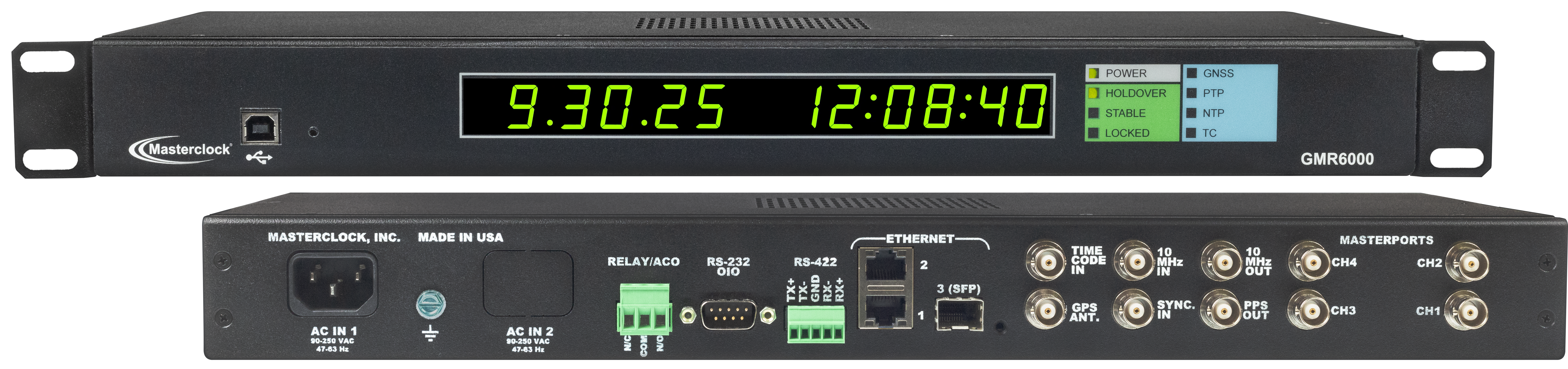
The GMR6000 features power redundancy, 4 Masterport outputs, 1 GigE interface, and a fast-disciplining rubidium oscillator capable of high-precision holdover. Learn more
About Dr. Demetrios Matsakis
 Dr. Demetrios Matsakis attended MIT as an undergraduate and received his PhD in physics from UC Berkeley, where he studied under the inventor of the maser and laser; and built specialized ones in order to observe interstellar dust clouds where stars are born. His first job was at the U.S. Naval Observatory, building water vapor radiometers and doing interferometry to observe quasars and galaxies at the edge of the observable universe. After developing an interest in clocks, Dr. Matsakis would spend the next 25 years working hands on with most aspects of timekeeping – from clock construction, to running the USNO’s Time Service Department, to international policy. He has published over 150 papers and counting, but gets equal enjoyment out of beta-testing his personal ensemble of Masterclock products.